
Identification of Development Poles on Brazilian Amazon Region and Analysis of the Geographic Accessibility
Identificação de Pólos de Desenvolvimento na Amazônia Brasileira e Análise da Acessibilidade Geográfica
Abstract
Identification of development poles within the regional planning is important for defining the nodes of a given transport network and plays the role of driving economic growth in a region. Nevertheless, such proceedings are complex, especially in some areas where there is a lack of data that could support studies of this nature, for example in the case of the Amazon region. Thus, this study aims to identify development poles using spatial analysis of production values of soya, coffee, wood, and mineral products like cassiterite, aluminum ore, iron ore and copper. In addition, the geographic accessibility analysis was carried out at these poles in order to identify the potential of the transport network to be structured. Results demonstrated that it is possible to build a dense transport network by identifying more development poles, which would increase the connectivity, allowing more intense exchange of flows and development of the region.
Keywords
Theory of development poles; spatial analysis, Amazon region.
Resumo
A identificação de pólos de desenvolvimento no planejamento regional é importante para definir os nós de uma determinada rede de transporte e desempenha o papel de impulsionar o crescimento econômico de uma região. No entanto, tais procedimentos são complexos, principalmente em algumas áreas onde faltam dados que possam subsidiar estudos dessa natureza, por exemplo, no caso da região amazônica. Assim, o presente estudo tem como objetivo identificar pólos de desenvolvimento por meio da análise espacial dos valores de produção de soja, café, madeira e produtos minerais como cassiterita, minério de alumínio, minério de ferro e cobre. Além disso, foi realizada a análise da acessibilidade geográfica nestes pólos com o objetivo de identificar o potencial da rede de transportes a ser estruturada. Os resultados demonstraram que é possível construir uma densa rede de transporte identificando mais pólos de desenvolvimento, o que aumentaria a conectividade, permitindo uma troca mais intensa de fluxos e desenvolvimento da região.
Palavras-chave
Teoria dos pólos de desenvolvimento; análise espacial; região amazónica.PLS-SEM.
Introduction
Large countries of the world as Brazil comprise under developing regions with great amounts of natural resources available such as the Amazon (Almeida et al., 2014, p. 90). Because the planning process does not account for all territories equally, these countries cannot achieve desirable levels of growth and development (Almeida et al., 2014, p. 90). In this case, the planning approach adopted mirrors inefficiency in regional planning, mainly in its three principal branches: transportation planning, infrastructure planning and territorial planning (Vasconcelos, 2000).
Transport planning defines the necessary facilities to ensure the transport of people and goods as also the transport systems (ANTP, 1999). Infrastructure planning defines the transport modes that could be used in the movement of people and products, it determines the means that provide the best conditions to be used. Finally, territorial planning is responsible for definitions and analyses of land use and occupation by the concepts of regional specialisation (Kraft et al, 1971), which, in accordance with (Lopes, 2001), should be included in the geographical context. When integrated ensures accessibility (Rodrigue, 2006, p. 22) “are a key element to geography transport, and to geography in general, since it is a direct expression of mobility either in terms of people, freight or Information”. According to the authors, efficient transportation systems offer high levels of accessibility (if the impacts of congestion are excluded), while less-developed ones have lower levels of accessibility (Rodrigue, 2006, p. 322).
Moreover, the absence of planning that is concerned with the location of activities in geographic space causes the main inefficiencies found in the regional planning process (Richardson, 1969). Such inefficiencies may cause a lack of identity to the role of the city in urban and regional planning. It is important that each city fulfills its social, cultural and economic role within regional development and in the national context. Thus, it could cause the dispersion of large urban centers and economic activities in the geographical space.
Dispersions, in this case, are mainly caused by incompatibilities between land use and transportation infrastructure available, which results in inefficient processes of regional economic development (Kraft et al, 1971; Banister et al, 2001 apud Almeida et al., 2014, p. 91). This situation could be solved by means of identifying important economic activities in the region so as to spot Poles of Economic Growth (Almeida et al., 2014, p. 91). Such poles would ignite economic growth aided by transportation infrastructure (Perroux, 1964). The combination of these elements (i.e., Poles of Economic Growth and transport infrastructure) would compose a complex transport network, which would contribute to accelerating regional economic growth (Taaffe et al, 1996 apud Almeida et al., 2014, p. 91).
Thus, this paper aims to identify the Development Poles in the Amazon Region through the spatial analysis of land use in relation to the main economics activities, assuming that the identification of such poles, is considered a prior activity to be carried out in development of a transport network (Almeida et al., 2014).
Basic literature review
Three main theoretical assumptions have been established in order to develop this study. The first one regarding development poles theory. The second aspect treated concerning geographic accessibility and network analysis. Finally, some features related to Spatial Analysis, especially Spatial Statistics, are presented.
Thus, the theory of development poles of Perroux and the economic region are was description by Almeida (2008) and Almeida et al. (2014), through François Perroux with developed the Growth Poles, and Development Poles Theory based on observation. Even though Perroux developed his theory around the industry because modern economy is led by industrial economic activity and also because he conducted his studies in industrialized countries, he extends the propulsive function to primary activities such as mining, forestry and farming.
From the economic point of view states, that space can be understood from three basic perspectives (Almeida et al., 2014, p. 91): (i) economic space as the content of a plan; (ii) economic space as a force field, and (iii) economic space as a homogeneous set of elements. Consequently, there are three types of economic regions: planned, polarised and homogeneous (Almeida et al., 2014, p. 91).
The concept of space as the content of a plan creates the planning regions. In this context, firms, public entities or any given economic agent have their own planning region, which both influences and it is influenced by their decisions. Regional development plans derive from planning regions framed by the public sector (Almeida et al., 2014, p. 91).
A city's power of attraction on the area that surrounds it, which results from its relationships with other areas or cities, causes areas of influence, and, consequently, polarised regions (Almeida et al., 2014, p. 91). The economy, by means of processes of trade, is, in essence, an activity that leads to regionalisation and determines the radius of a city’s area of influence. Thus, highways expand around it, which increases the city’s power of attraction (Almeida et al., 2014).
In short, François Perroux conceives poles as the dynamic economic center of a region, country or continent (Almeida et al., 2014, p. 92). Growth stemming from poles is felt throughout their surroundings, as they create flows from the surrounding regions toward the center as well as the other way around. Regional development is always linked to its pole's development trends (Almeida et al., 2014, p. 92).
The Notion of Accessibility in Network Analysis
The degree to which two places (or points) on the same surface are connected and integral accessibility is “the degree of interconnection with all other points on the same surface” (Prasad, 2020, p. 2). Accessibility is defined as the measure of the capacity of a location to be reached by, or to reach different locations (Rodrigue et al, 2006, p. 304). Therefore, the capacity and the structure of transport infrastructure are key elements in the determination of accessibility (Rodrigue et al, 2006, p. 304).
However, identify four interrelated issues, which must be resolved: the degree and type of disaggregation (Spatial, socio-economic and the purpose of the trip or the type of opportunity); the definition of origins and Destinations; the measurement of travel impedance (commonly measured by distance or time) and the measurement of attractiveness (Handy, 1997).
All places are not equal because some are more accessible than others, which implies inequalities (Rodrigue et al, 2006, p. 322). The notion of accessibility consequently relies on two core concepts, and this depends on location and time. The location where the relativity of places is estimated in relation to transport infrastructures, since they offer the mean to support movements. The distance, which is derived from the connectivity between locations (Rodrigue et al, 2006, p. 322). The connectivity can only exist when there is a possibility to link two locations through transportation. It expresses the friction of space (or deterrence) and the location which has the least friction relative to others is likely to be the most accessible. Commonly, distance is expressed in units such as in kilometers or in time, but variables such as cost or energy spent can also be used (Rodrigue et al, 2006, p. 322).
Geographic Accessibility
Geographic accessibility considers that the accessibility of a location is the summation of all distances between other locations divided by the number of locations (Rodrigue et al. 2006, p. 326). In this measure of accessibility, the most accessible place has the lowest summation of distances (Equation 1) (Rodrigue et al. 2006, p. 326).
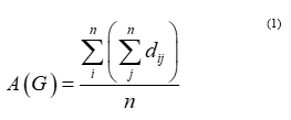
where A (G) geographical accessibility matrix;
dij: shortest path distance between location i and j;
n: number of locations.
Spatial Analysis
Spatial analysis could be understood as a technique to describe what kind of patterns there is in spatial data and to make relationships between several geographic variables (Câmara et al., 2001). Therefore, the understanding of how data is ordered in space and its interrelationship is a function of spatial analysis.
Given the importance of analyzing spatially attributes related to the development and growth of economic activities and the potential that may be found in spatial analysis tools, it is necessary to use this tool in order to identify the location of development poles. Thus, some concepts are presented in order to understand the analyses carried out in the development of this study.
Spatial Analysis (SA): concepts, features and tools
The basic principles of Spatial Analysis involve the way in which data on health, environment, geology, agronomy and transport are organized in space, and what is the relationship between them (Henrique, 2004).
With regard to the analysis of spatial relations it could be highlighted analysis of accident patterns and diagnosis of transport systems (Henrique, 2004). In this case, some tools are used, among which there is a proposal that deserves attention, namely, which is constituted by four different tools: selection, manipulation, exploratory analysis and confirmatory analysis (Anselin, 1996).
Spatial Statistics, which encompasses the mathematical tool, helps the planner to establish quantitative criteria for grouping or dispersing spatial data, besides obtaining the degree of spatial dependence between observations (autocorrelation) (Teixeira, 2003).
Spatial Statistics
The main purpose of spatial statistics is characterise spatial patterns. These patterns cause measurement problems, called spatial effects, such as spatial dependence and spatial heterogeneity, which affect the operation of traditional statistical methods as well as behavioural models (Portugal, 2012).
The basic principle of the Spatial Statistics is the first law of geography (Teodorovic, 1986). The author says that everything is related to everything else. But near things are more related than distant things (Orlando e Togo, 2012, p. 2).
Exploratory Spatial Data Analysis (ESDA)
The spatial autocorrelation or spatial dependence is the focus of this study while it is necessary to identify regions that have spatial dependence and are statistically significant. In that case, the spatial analysis is made by global and local statistics using Indicator of Spatial Dependence (Moran’s I), Local Indicator of Spatial Association (LISA) and scatter diagrams (BoxMap, LisaMap and MoranMap). All of these maps and indicators are parts of ESDA techniques (Exploratory Spatial Data Analysis) whose function is assisting in the identification of objects with high and low values, transition areas and atypical cases.
Positive spatial dependence occurs when an event influences the occurrence of another similar to its surroundings, generating an agglomerated distribution. If the same event influences or prevents the occurrence of another around it, it is said there is a negative autocorrelation, with approximately equidistant distribution of events (Souza, 2005).
It could be seen that spatial analysis techniques may significantly increase the ability to understand spatial patterns associated with area data, especially when referring to social indicators that have global and local spatial autocorrelation. Exploratory tools, such as Moran Map, are useful for showing spatial aggregations and indicating priority areas in terms of public policies (Souza, 2005).
- Elements and Relations of the ESDA
The basic elements that constituted the ESDA techniques are: proximity matrix (W), deviation vector (Z) and the weighted mean vector. The deviation vector may be calculated using the Equation (2).
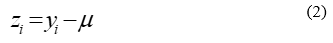
where ![]() deviation vector;
deviation vector;
![]() attribute value;
attribute value;
![]() overall average.
overall average.
The vector of weighted averages may be calculated using the Equation (3).
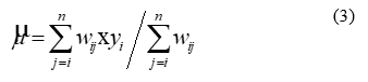
Where ![]() weighted average;
weighted average;
 Spatial proximity matrix;
![]() attribute value.
attribute value.
b) Global and Local Space Autocorrelation Indicators
The global autocorrelation indicators evaluate one of the main features of the exploratory analysis, the spatial dependence. Such indicators aim to estimate how much a value observed in a given area depends on this same variable in neighboring locations, as a result we have a unique spatial association value for the entire dataset (Henrique, 2004).
Regarding Moran's I, this measures the spatial autocorrelation calculated by means of equation 4 whose values can vary between -1 and +1.
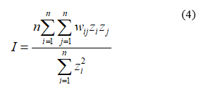
Where I: Moran’s I;
n: is the number of observations (points or polygons);
![]() difference between the value of the attribute in place i and the average of all attributes;
difference between the value of the attribute in place i and the average of all attributes;
![]() difference between the value of the on-site neighbor’s attribute in place j and the average of all attributes;
difference between the value of the on-site neighbor’s attribute in place j and the average of all attributes;
![]() is a weight indexing location of i relative to j.
is a weight indexing location of i relative to j.
The Moran Scatterplot is a useful visual tool for exploratory analysis, because it enables you to assess how similar an observed value is to its neighboring observations. Its horizontal axis is based on the values of the observations and is also known as the response axis. The vertical Y axis is based on the weighted average or spatial lag of the corresponding observation on the horizontal X axis (Anselin, 1996). The Moran Scatterplot is defined as a two-dimensional graph divided into four quadrants, allowing to analyse the spatial variability behaviour (Lopes, 2005). It is instructive to consider each quadrant of the plot. In the upper-right quadrant are cases where both the value and local average value of the attribute are higher than the overall average value. Similarly, in the lower-left quadrant are cases where both the value and local average value of the attribute are lower than the overall average value. These cases confirm positive autocorrelation. Cases in the other two quadrants indicate negative autocorrelation. Depending on which groups are dominant, there will be an overall tendency towards positive or negative (or perhaps no) autocorrelation (Balyani et al., 2017).
The local indicators of spatial autocorrelation allow us to analyses spatial association values in detail (Equation 5).
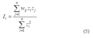
Where Ii: local indicator of spatial autocorrelation;
z i : difference between the value of the attribute in place i and the average of all attributes;
wij : is a weight indexing location of i relative to j.
The LISA Map and Moran Map are useful because with them it is possible to identify regions that present local correlation significantly different from the other data, highlighting particular spatial dynamics, which deserve more detailed studies (Lopes, 2005).
Methodology to Identify Development Poles
The methodology for the identification of development poles is constituted for six (6) steps: step 1 – definition of study area: Amazon Region; step 2 – diagnosis of the regional economy; step 3 – building a geographic database; step 4 – identifying potential development pole areas; step 5 – applying the spatial statistics tools to identify the development poles; step 6 – geographic accessibility analysis.
Identification of Development Poles on Amazon Region
Step 1: Definition of Study Area - Brazilian Amazon Region
The Brazilian Amazon Region covers an area of 5,217,423 km2. The region encompasses the entire Northern region, a great deal of the Midwestern region and some of the Northeast (Almeida et al., 2014). The figure 1 shows the geographical extent of Amazon Region being considered in this study, which comprises nine states (and 808 towns): Acre, Amapá, Amazonas, Mato Grosso, Pará, Rondônia, Roraima, Tocantins and part of the Maranhão state. The population of the states of the Amazon Region amounted to 28.280,974 people (IBGE, 2000), which corresponded to 13.6% of the Brazilian population.
Among the peculiarities that Amazon Region presents, the low demographic density stands out, which still reflects the low territorial occupation, and the great amount of available natural resources (Théry, 1999).
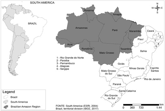
Figure 1. Study Area, Brazilian Amazon Region.
Step 2: Diagnosis of the Regional Economy
In this step a diagnosis has been done regarding the regional economy. In that context, it is possible to identify that Amazon Region's economy is supported by mining, forestry and farming (agriculture). These activities are carried out by means of making use of a few unique local products. There are twenty goods supporting the economy, which can be classified in following groups of activities (Almeida et al., 2014, p. 93):
Mining: these activities are characterized by the extraction of various minerals, such as: iron ore, oil, aluminum ore, kaolinite, natural gas and tin. However, iron ore is one of the most important products of the region; Forestry: these activities are characterized by the extraction and/or processing timber and latex, mainly; Farming (agriculture): a few crops are grown in the Amazon Region, such as: soybean, rice, cassava, cotton, corn and coffee. Among these, more emphasis is given to soybean, rice and cassava.
The definition of these products followed the proposal of Almeida e. al. (2014), which used the ABC Analysis of the production value of the most significant products for the economy of the Amazon region.
Step 3: Building a Geographic Database
A GIS-based database was built using data gathered during the diagnosis stage. One type of layer was manipulated, namely, an area layer, representing 808 towns of the study area was created. Thus, A layer is created for each product identified in the diagnosis stage; in total, twenty layers were created. Information was attached to each layer regarding the production value and the amount produced in each town where such economic activities are undertaken (Almeida et al., 2014, p. 93).
Step 4: Identifying Potential Development Pole Areas
According Almeida et al. (2014, p. 94), in order to identify the potential areas, two activities were conducted: thematic maps of the distribution of the chosen variable were created; and analyses of spatial distribution were conducted on those maps to identify geographic areas encompassing sets of towns that have highest production values.
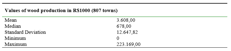
Table 1 presents the statistics on the values of wood production, whose results will serve as parameters for the analyses that will follow. Note the mean and median values are low in comparison to the maximum value of the universe studied. Thus, the large amount of the towns has low values for the variable Value of Production of the wood.
Table 1.
Statistics of the Values of Production, 2016.
Thus, maps were generated to present the development poles by analysis products. The first poles analyzed regarding the wood (Figure 2), coffee (Figure 3) and soybean (Figure 4). Analyses of spatial distribution were conducted on maps to identify geographic areas encompassing sets of towns (clusters) that have the highest production values (Almeida et al., 2014). The result for the wood showed the poles are located mainly in the state of Pará, two clusters in Portel and Paragominas, Oriximiná and Santarém (far north), in the Aripuanã on state of Mato Grosso (far south), with high production values in the Lábrea on state of Amazonas and Porto Velho on state of Rondônia.
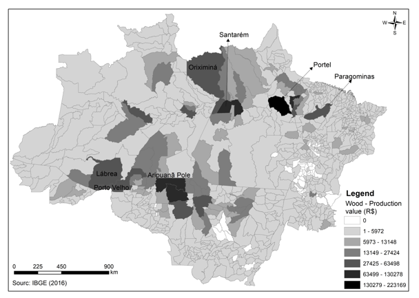
Figure 2. Spatial localization of the development poles - wood production.
Coffee and soybean present high concentrations. Figure 3 presents the spatial localization of the development poles relating to the coffee, which could be identified in the southwest part, in the state of Rondônia. On the other hand, Figure 6 shows that development poles concerning the soybean are concentrated in the south part, in the state of Mato Grosso. Finally, spatial analyses were made on such maps with the purpose of identifying spatial cuts made up of groups of towns that have the highest and lowest production values.
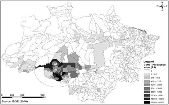
Figure 3. Spatial localisation of the development poles - coffee bean production.
The soy production is one of the most important economic activities in the Brazilian Amazon, where it is mechanised and takes place at industrial scales (Rausch, 2016, p. 2). In this system the producer is supported by a conglomeration of institutions, industry of inputs, crushers and refiners, derivatives industry, distributors, credit institutions, research, technical assistance, etc (Oliveira Junior, 2013).
Thereby, "since 1997 the Madeira - Amazonas inland water navigation connects the ports of soybean transshipment of the Maggi and Cargill groups (hegemonic agents), i.e., it connects the city of Porto Velho to Itacoatiara and to Santarém” (Silva, 2013). Thus, soybean grains produced in the state of Rondônia and in the northwest of Mato Grosso state are transported through this waterway network for Europe and China (Silva, 2014). These regions, in a first analysis, can potentially be considered as Development Poles. However, it is necessary to confirm by spatial analysis techniques whether such areas are Developmental Poles.
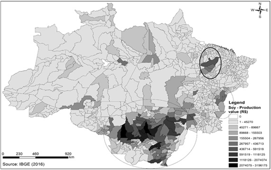
Figure 4. Spatial localisation of the development poles - soybean production.
Step 5: Applying the Spatial Statistics Tools to Identify Development Poles
According Almeida et al. (2014), this step resorts to spatial statistics indicators and maps, which provide a basis for decision-making. The first indicator we calculated was Moran's I, which expresses the degree of homogeneity or heterogeneity of the study area. Next, Box Map was created to verify the relationship of the variable in space with its neighbors. Finally, the Moran Scatterplot was created to identify statistically significant areas that represent the development poles.
Thus, detailed analysis has been done for wood, coffee and soybean. Spatial analysis of groups was determined for each of these products, which expressed the degree of homogeneity or heterogeneity of the studied area. BoxMap and Moran Map were developed in order to analyse the production values of these three goods. As seen in the literature review, BoxMap represents the Moran spreading diagram and Moran Map associates the significance of the Moran's I with the Moran spreading diagram.
The Figure 5 presents the spatial patterns of the variables of wood production value. The Box Map presents how all the areas of the region are linked. Using the Box Map it is possible to notice there is a well-defined cluster of areas with the same aggregation pattern (Almeida et al., 2014). The darker-colored aggregate areas are related more strongly (High-High) due to high attribute values coinciding with areas previously identified as possible PD.
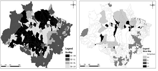
Figure 5. Box Map (a) e Moran Map (b) of the Amazon Region for variable Production Value Madeira.
The identification of areas that are significantly greater or equal to 95% confidence interval is given through the Moran Map (Figure 5b). The areas classified as HH (of Moran Map) have a strong correlation and are significant, while others do not have such a pattern because they are in a region of instability. Figure 5b presents the Development Poles in the Amazon Region under the timber production approach.
Similar analysis was performed for soybean and coffee. Thus, the spatial patterns of soybean occurrence revealed a cluster in the state of Mato Grosso, at the central-north region (Fig. 6). The presence of high production values of soybean coinciding with 95% of confidence interval, this was observed through Moran Map (Fig. 6b). Comparing this result with the values presented by (Almeida, 2008), it was observed the consolidation of the area of soybean cultivation in the central-north region of the state of Mato Grosso.
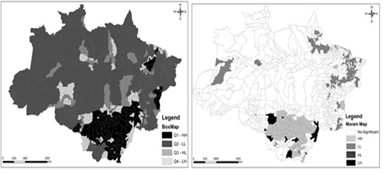
Figure 6. Box Map (a) e Moran Map (b) of the Amazon Region for Variable Value of Soybean Production.
The coffee beans cultivation was identified only in the state of Rondônia (Fig. 7). Therefore, clusters with 95% of confidence interval in this area (Fig. 7b). The low value grouping for coffee production coincides with no significant areas. The cluster of cities with high significance by the Box Map (Fig. 7a) in the northwest region of Mato Grosso (indicated by the circle in the figure) did not present significance.
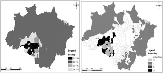
Figure 7. Box Map (a) e Moran Map (b) of the Amazon Region for Variable Value of Coffee bean Production.
The poles characterised by iron, tin, aluminum and copper production values are illustrated in Fig. 8. Thus, Pará, Amazonas and Rondônia stand out as producers of ores.
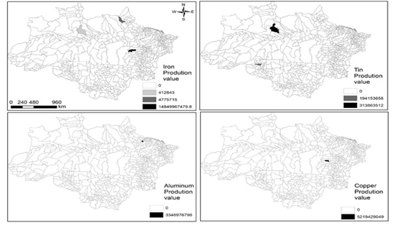
Figure 8. Spatial localisation of Iron, Tin, Aluminum and Copper for PD.
Step 6: Geographic Accessibility Analysis
The Geographic Accessibility revealed with development poles integrates in Amazon Region by OD Cost Matrix of the Network Dataset. This function uses determined impedance. For the author, accessibility should be measured by the frequency of trips according to classes of expenditure (Macke, 1974). In this case, time or distance. The speeds were estimated from the research developed by (Almeida et al, 2014).
Table 2 shows the geographical accessibility of the development poles in the Amazon Region. In table 2 it is possible to identify the Development Poles and the position that they occupy in the ranking. This ranking was defined using the geographical accessibility matrix considering the minimum paths between the poles of development. Although the graphical representation is made in straight lines, the values stored in the attribute table represent the actual (topological) distance of the network. Thus, this data represents the matrix found for the lowest cost paths from each source to the other destinations. The output shape was set to produce straight lines. The resulting matrix data was used in the accessibility maps (Fig. 10, 11, 12, 13, 14 and 15).
Table 2.
Geographic Accessibility in Amazon Region.
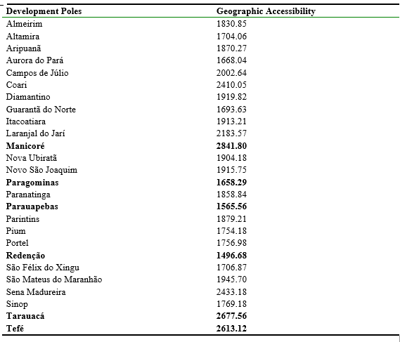
Thus, the results showed the poles of Redenção (1496.68km), Paraupebas (1565.56km) and Paragominas (1658.29km), all of them localised in the state of Pará, are the most accessible. These three poles are associated with the national network and have shown diversification of modes in terms of accessibility.
On the other hand, the least accessible poles are Manicoré (2841,80km), Tarauacá (2677,56 km) and Tefé (2613,12km). Regarding Manicoré, despite its centralised location, there is only one type of transportation mode. In case of the pole of Tarauacá, the distance possibly was a determinant factor for its difficult access, since it is the point more to the extreme west in the region. Similar analyses may be associated with access to Tefé, also distant from other poles.
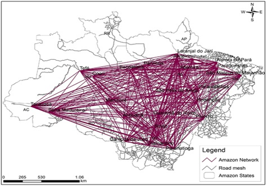
Figure 9. Geographical accessibility between the Poles de Development in the Amazon.
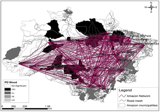
Figure 10. PD of wood (Moran Map) vs. accessibility.
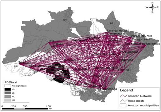
Figure 11. PD of coffee bean (Moran Map) vs. accessibility.
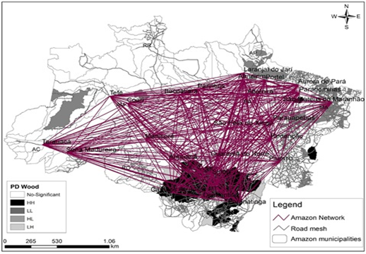
Figure 12. PD of soybean (Moran Map) vs. accessibility.
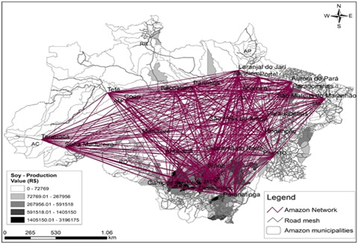
Figure 13. PD of soybean (production data in R$) vs. accessibility.
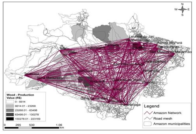
Figure 14. PD of wood (production data in R$) vs. accessibility.
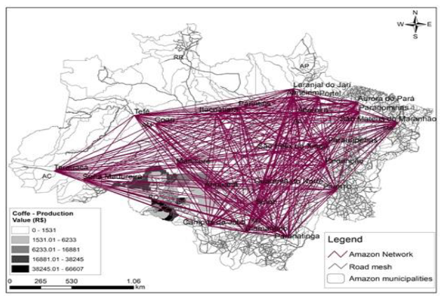
Figure 15. PD of coffee bean (production data in R$) vs. accessibility.
Conclusions
This study aimed at applying the principles of the spatial analysis tools to assist the regional planning process, specifically concerning the integration of transport, territory and economy. Initially, the development poles were identified. Then, these poles was analysed under geographic accessibility approach. Consequently, the Spatial Analysis and the Geographic Accessibility Matrix proved to be important tools for observing the inter-relationship among transporte and territory in order to assist in the construction of a transport network that promotes regional economic growth.
From the research it was possible to conclude that:
- The results corroborate the fact that adequate planning of the transport system is necessary to favor the connectivity of the development poles;
- In addition, a survey concluded that the municipality of Redenção, in the state of Pará, is the most accessible pole, expressive concentrations of soybean cultivation;
- The least accessible poles are Manicoré (2841, 80km), Tarauacá (2677, 56km) and Tefé (2613, 12km). Regarding Manicoré, despite its centralised location, there is only one type of transportation mode. In case of the pole of Tarauacá, the distance possibly was determinant factor for its difficult access, since it is the point more to the extreme west in the region;
- It was in the southern portion where it was identified however, its accessibility makes it difficult to produce, which is made exclusively by highways to the bulk port of the city of Porto Velho.
- It is necessary to present some limitations of this study, namely:
- There is no disaggregated data representing smaller areas of the Amazon Region which compromises the accuracy of the results achieved.
- Second-hand data was used to identify poles;
- There is lack of availability for conducting field research.
- The following recommendations can guide future studies on the topic:
- Economic feasibility analysis of the deployment of a transport network considering the development poles as network nodes;
- Propose a further study that could consider the propagating effect of the poles in the territory;
- Sensitivity analysis considering the emergence of new poles.